Quantifying Evidence (2): Evidence Is Limited By How Much a Study Can Be Trusted

In part 1, we defined evidence and showed that evidence across independent studies can be aggregated by addition; if Alice’s results provide 2 units of evidence and Bob’s results provide 3 units of evidence then we have a total of 5 units of evidence. The problem with this is that it doesn’t account for our intuition that single experiments cannot be trusted too much until they are replicated. 10 congruent studies each reporting 2 units of evidence should prevail over one conflicting study showing -20 units of evidence.

Let’s try to model this by assuming that every experiment has a chance of being flawed due to some mistake or systematic error. Each study can have its own probability of failure, in which case the results of that experiment should not be used at all. This is our first assumption: that any result is either completely valid or completely invalid. It is a simplification but a useful one.

We define trust (T) in a particular study as the logarithm of the odds ratio for the being valid versus being invalid. In formal terms:

$T = (\text{subjective trust in a particular result}) = \log_{10}\left(\dfrac{Pr(\text{valid})}{Pr(\text{invalid})}\right) = \log_{10}\left(\dfrac{Pr(V)}{Pr(\overline{V})}\right)$

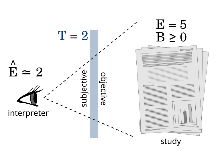
A trust T=2 corresponds to a belief that the odds the outcome being flawed is 1 to 100. T=3 corresponds to an odds of 1 to 1000. In my view, 1<T<3 is reasonable for the typical study. But trust is something subjective that cannot be objectively calculated. Much like priors, it depends on the person sitting outside of the study interpreting its results.

Take a study with data $D$ that reports evidence $E$ . That study can either be valid or invalid (represented by $V$ and $\overline{V}$ ). The reported evidence was calculated under the assumption that the study was valid. So:

$E = (\text{reported evidence}) = \log_{10}\left(\dfrac{Pr(D | H_1 \& V)}{Pr(D | H_2 \& V)}\right)$

$\begin{align*} \\ \Rightarrow \begin{cases} P(D|H_1\&V) = (P(D|H_1\&V)+P(D|H_2\&V)) / (1 + 10^{-E}) \\ \\ P(D|H_2\&V) = (P(D|H_1\&V)+P(D|H_2\&V)) / (1 + 10^{E}) \end{cases} \end{align*}$

From the perspective of an observer interpreting a study with trust $T$ , we can calculate the effective evidence, $\hat{E}$ .

$\begin{align*} \Hat{E} &= (\text{effective evidence}) = \log\left( \dfrac{Pr(D | H_1)}{Pr(D | H_2)} \right) \\ &= \log\left( \frac{P(D|H_1\&V)P(V) + P(D|H_1\&\overline{V})P(\overline{V})}{P(D|H_2\&V)P(V) + P(D|H_2\&\overline{V})P(\overline{V})} \right) \\ &= \log\left( \frac{P(D|H_1\&V)\times 10^T + P(D|H_1\&\overline{V})}{P(D|H_2\&V)\times 10^T + P(D|H_2\&\overline{V})} \right) \\ &= \log\left( \frac{(P(D|H_1\&V)+P(D|H_2\&V))(1 + 10^{-E})^{-1} 10^T + P(D|H_1\&\overline{V})}{(P(D|H_1\&V)+P(D|H_2\&V))(1 + 10^{E})^{-1} 10^T + P(D|H_2\&\overline{V})} \right) \end{align*}$

We define G as the resulting evidence in case the study is invalid.

$G = log\left(\frac{P(D|H_1\&\overline{V})}{P(D|H_2\&\overline{V})}\right)$

$\begin{align*} \\ \Rightarrow \begin{cases} P(D|H_1\&\overline{V}) = (P(D|H_1\&\overline{V})+P(D|H_2\&\overline{V})) / (1 + 10^{-G}) \\ \\ P(D|H_2\&\overline{V}) = (P(D|H_1\&\overline{V})+P(D|H_2\&\overline{V})) / (1 + 10^{G}) \end{cases} \end{align*}$

$\Rightarrow \Hat{E} &= \log\left( \dfrac{(1 + 10^{-E})^{-1} 10^T + \dfrac{P(D|H_1\&\overline{V})+P(D|H_2\&\overline{V})}{P(D|H_1\&V)+P(D|H_2\&V)}(1 + 10^{-G})^{-1}}{(1 + 10^{E})^{-1} 10^T + \dfrac{P(D|H_1\&\overline{V})+P(D|H_2\&\overline{V})}{P(D|H_1\&V)+P(D|H_2\&V)}(1 + 10^{G})^{-1}} \right)$

Here we are going to make another simplification: The second assumption is that if a study is invalid, it provides no evidence for or against H₁ versus H₂. In other words G = 0. This means $P(D|H_1\&\overline{V})$ = $P(D|H_2\&\overline{V})$ = $P(D|H_{1 \lor 2}\&\overline{V})$ . Substituting for these values we get:

$\begin{align*} \Hat{E} &= \log\left( \dfrac{(1 + 10^{-E})^{-1} 10^T + \dfrac{P(D|H_1\&\overline{V})+P(D|H_2\&\overline{V})}{P(D|H_1\&V)+P(D|H_2\&V)} \times \dfrac{1}{2}}{(1 + 10^{E})^{-1} 10^T + \dfrac{P(D|H_1\&\overline{V})+P(D|H_2\&\overline{V})}{P(D|H_1\&V)+P(D|H_2\&V)} \times \dfrac{1}{2}} \right) \\ &= \log\left( \dfrac{(1 + 10^{-E})^{-1} 10^T + \dfrac{P(D|H_{1,2}\&\overline{V})}{P(D|H_1\&V)+P(D|H_2\&V)}}{(1 + 10^{E})^{-1} 10^T + \dfrac{P(D|H_{1,2}\&\overline{V})}{P(D|H_1\&V)+P(D|H_2\&V)}} \right) \end{align*}$

And to simplify the above formula we define another term: believability. Believability (B) is defined below.

$B = log \left( \dfrac{P(D|H_1\&V)+P(D|H_2\&V)}{P(D|H_{1 \lor 2} \&\overline{V})} \right)$

Substituting B we get the following:

$\begin{align*} \Hat{E} &= \log\left( \dfrac{(1 + 10^{-E})^{-1} 10^T +10^{-B}}{(1 + 10^{E})^{-1} 10^T + 10^{-B}} \right) = \log\left( \dfrac{(1 + 10^{-E})^{-1} 10^{(T+B)} +1}{(1 + 10^{E})^{-1} 10^{(T+B)} + 1} \right) \\ &= \log\left( \dfrac{ \left(\dfrac{10^E + 1}{10^{E}}\right)^{-1} 10^{(T+B)} +1}{(1 + 10^{E})^{-1} 10^{(T+B)} + 1} \right) = \log\left( \dfrac{ \left(\dfrac{10^{E}}{1 + 10^E}\right) 10^{(T+B)} +1}{ \dfrac{1}{1 + 10^{E}} 10^{(T+B)} + 1} \right) \\ &= \log\left( \dfrac{ 10^{E} \times 10^{(T+B)} + (1 + 10^{E})}{ 10^{(T+B)} + (1 + 10^{E})} \right) = \log\left( 10^{E} \times \dfrac{ 10^{(T+B)} + 10^{-E} + 1}{ 10^{(T+B)} + 10^{E} + 1} \right) \\ &= E + \log\left( \dfrac{ 10^{(T+B)} + 10^{-E} + 1}{ 10^{(T+B)} + 10^{E} + 1} \right) \end{align*}$

It’s alright if you didn’t closely follow the math up to here. What is important is that we now have a formula for calculating effective evidence $(\hat{E})$ based on reported evidence $(E)$ , trust $(T)$ , and believability $(B)$ .

$\Hat{E} = E + \log\left( \dfrac{ 10^{(T+B)} + 10^{-E} + 1}{ 10^{(T+B)} + 10^{E} + 1} \right)$

The reported evidence $(E)$ is an objective number we get from the study. Trust $(T)$ is a subjective quantity that the subjects interpreting the study must determine for themselves, independent of the outcome of the study. Believability is a bit more complex. Believability is a number ascribed to a particular outcome or observation, much like evidence is. But in contrast to evidence, believability cannot be determined objectively. This is because of the term $P(D|H_{1,2}\&\overline{V})$ which has to be determined by the interpreter; it is subjective and can vary for different people. I will write more about believability in the next part of this series. (Suffice it to say that a study can be designed to guarantee a believability of B≥0).

	meaning	subjective/objective	dependence on study	range
Evidence (E)	amount of evidence provided by the study’s outcome	objectively calculated	depends on outcome	positive (in case the data favors H1) or negative (in case it favors H2)
Trust (T)	amount of trust placed in a study prior to seeing the outcome	determined subjectively	independent of outcome	typically a positive number between 1 and 3
Believability (B)	amount of believability ascribed to the outcome of an experiment	determined subjectively, but a lower bound can sometimes be objectively calculated	depends on outcome	negative if the outcome is an indication that the study is likely flawed. The ideal study guarantees that B≥0.

To gain a better understanding about how the above formula works, I made the following plot.

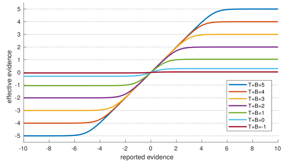
Effective evidence begins to grow linearly with respect to reported evidence. But it plateaus at (T+B). In other words, evidence is effectively limited by how much a study can be trusted plus the believability of the study’s outcome. To first approximation, the magnitude of effective evidence is roughly equal to min(|E|, T+B). This approximation is least accurate when |E| ≈ T+B or when T+B < 1.

This formalizes our intuition that no single study can be used to decisively confirm or deny a hypothesis, no matter how strong the evidence turns out to be in that study. The amount of trust one places in a study limits the amount of evidence that can be acquired from it. For example, if you place a trust of T=1.5 in the typical paper, no single study can convince you by more than 1.5 units of evidence (assuming B=0; more on believability later). You would need to add the effective evidence ( $\hat{E}$ ) from multiple independent studies to establish that there is higher than 1.5 units of evidence for something. This aspect of our framework is nice, because astronomically large or small values are commonplace when working with likelihood ratios. But by accounting for trust, extremely large amounts of reported evidence are not extremely informative.

A meta analysis of multiple studies can be done by calculating the effective evidence for each study and then summing the values. 10 studies that each report 2 units of evidence will almost certainly prevail over one [conflicting] study that reports -20 units of evidence, given that no study can reasonably be trusted with T≥20. If T = 3 and B = 0, then the overall evidence in this case is is 10×2-3 = 9. (Each of the first 10 studies will have an effective evidence of 2 and the single conflicting study will have an effective evidence of -3).

Now, here is a problem that will lead us to the next part. How do we deal with believability? From the perspective of a researcher, we would like to maximize it since it limits the evidence that can be deduced from a study.

If the outcome of an experiment is a continuous value, then all the probabilities in the above formulas can get infinitesimally small. The numerator depends on the person evaluating our study and can be infinitely large for some inconveniently skeptical interpreter. So there is no limit to how negative believability can get! If believability is not dealt with in a study, there is no guarantee that a skeptical interpreter can take away any information from that study. What can be done to guarantee something like this will not happen? I will discuss this in part 3.