

Suppose I tell you that only 1% of people with COVID have a body temperature less than 97°. If you take someone’s temperature and measure less than 97°, what is the probability that they have COVID? If your answer is 1% you have committed the conditional probability fallacy and you have essentially done what researchers do whenever they use p-values. In reality, these inverse probabilities (i.e., probability of having COVID if you have low temperature and probability of low temperature if you have COVID) are not the same.
To put it plain and simple: in practically every situation that people use statistical significance, they commit the conditional probability fallacy.
When I first realized this it hit me like a ton of bricks. P-value testing is everywhere in research; it’s hard to find a paper without it. I knew of many criticisms of using p-values, but this problem was far more serious than anything I had heard of. The issue is not that people misuse or misinterpret p-values. It’s something deeper that strikes at the core of p-value hypothesis testing.
This flaw has been raised in the literature over and over again. But most researchers just don’t seem to know about it. I find it astonishing that a rationally flawed method continues to dominate science, medicine, and other disciplines that pride themselves in championing reason and rationality.
What Is Statistical Significance?
This is how hypothesis testing is done in today’s research. When researchers decide to test a hypothesis, they collect data — either from experiments they themselves design or from observational studies — and then test to see if their data statistically confirms the hypothesis. Now, instead of directly testing the hypothesis, they attempt to rule out what is called the null hypothesis. Think of the null hypothesis as the default.
For example if I want to show that “turmeric slows cancer”, I rule out the null hypothesis that “turmeric has no affect on cancer”. The null hypothesis can be ruled out by showing that the data is unlikely to have occurred by chance if the null hypothesis were true. In our example, it would be something like saying “it is unlikely that this many people would have recovered if turmeric has no affect on cancer“. In other words, the data is statistically significant.
To quantify statistical significance, we use a measure called the p-value. The p-value for observing some data, represents the probability of getting results as extreme as what was observed under the null hypothesis. The lower the p-value, the less likely it is for the observations to have occurred by chance, hence the more significant the observations. So, in the turmeric treatment example, I may obtain p=0.008 which means the probability of having at least that many patients recover by chance would have been 0.8% (assuming the null hypothesis: that turmeric actually has no effect). Since it is so unlikely for us to have obtained these results by chance, we say these results are significant and it is therefore reasonable to conclude that the drug does indeed affect cancer.
The standard method for p-value testing is to choose a significance threshold before looking at the data. It is typical to set the threshold at p<0.05, or sometimes p<0.01. If the p-value is less than the threshold, the data is considered to be statistically significant and the null hypothesis is rejected. Otherwise, the study is considered to be inconclusive and nothing can be said about the null hypothesis.
The Fundamental Flaw
A rational observer rules something out if its probability is low. So perhaps we can all agree that it is rational to reject the null hypothesis (H0) if its probability falls below some threshold, say 1%. Now if we gather some new data (D), what needs to be examined is the probability of the null hypothesis given that we observed this data, not the inverse! That is, Pr(H0|D) should be compared with a 1% threshold, not Pr(D|H0). In our current methods of statistical testing, we use the latter as a proxy for the former.
The conditional probability fallacy is when one confuses the probability of A given B with the probability of B given A. For example, the probability of that you are sick if you have a fever is not equal to the probability that you have a fever if you are sick; if you have a fever you are very likely sick, but if you are sick the chances of you having a fever are not equally high.
By using p-values we effectively act as though we commit the conditional probability fallacy. The two values that are conflated are Pr(H0|p<α) and Pr(p<α|H0). We conflate the chances of observing a particular outcome under a hypothesis with the chances of that hypothesis being true given that we observed that particular outcome.
Now how exactly can this fallacy lead to incorrect inference? If we overestimate the probability of the null hypothesis, well, that is not such a serious problem; the study will be declared “inconclusive”. It is a more serious problem if we underestimate the probability of the null hypothesis and reject it when we shouldn’t have.
There are two sources of irrational hypothesis rejection: 1) high prior probability for the null hypothesis and 2) low statistical power.
The Priors (or Base Rate)
One factor that can lead to irrational hypothesis rejection is the the base rate (or prior probabilities). There is an illustrating examples of this on the most recent Wikipedia entry on “Base Rate Fallacy”.
The more we test hypotheses that are unlikely to be true begin with, the higher the rate of error. For example, if the number of benign drugs that we test outnumbers the number of effective drugs, we will end up declaring too many drugs as effective.
A common argument that is raised in defense of p-values is that priors are inaccessible, subjective, and cannot be agreed upon. How does one measure the probability of a hypothesis independent of data? For example, how does one objectively find the probability of drugs effectiveness prior to any data analysis? This is a fair point. But priors are not the only factor that lead to irrational hypothesis rejection.
It’s Not Just About Priors
Statistical power is the probability of correctly rejecting the null hypothesis. Typically, the larger the sample size in a study, the higher its statistical power (i.e. the higher the chance of being able to declare statistical significance in the data). Rarely do scientists ever calculate statistical power or impose any constraints on it. Researchers worry less about statistical power because we [incorrectly] think that the only harm in low powered tests is obtaining inconclusive results. (Think of the case we test a new drug and don’t find evidence that it cures cancer while it actually does). That seems like a problem that can be fixed by collecting more data and increasing the population size in future studies.
What we really want to avoid is what is called type I errors, i.e. incorrectly rejecting the null hypothesis, not type II errors, i.e. failure to correctly reject the null hypothesis. Concluding that a drug cures cancer when it actually has no effect (which can have awful consequences) versus failure to find evidence that a drug cures cancer when if actually does (which is bad but can be corrected through more research). Since we are primarily concerned with type I errors, we impose constraints on the significance levels of our tests. So we set a 0.05 threshold for p-values if a 5% type I error rate is deemed acceptable. However, this line of reasoning is problematic. As I show below, low statistical power can lead to more frequent type I errors.
Calculating the Error Rate
Let us calculate the probability of unjustifiably rejecting the null hypothesis. Remember, a rational person sets a threshold for Pr(H0|p<0.01), not Pr(p<0.01|H0), given they consider 1% probability to be an appropriate threshold for rejecting a hypothesis.
Assume that we have designed a test with statistical significance threshold α and statistical power 1-β to reject the null hypothesis H0. What is the probability that a conclusive study commits a type I error? In other words what is the probability that H0 is true given that the data passes our significance test (p<α)? Using Bayes’ rule, we have:

Let us set the probability of committing a type I error to be less than e and rearrange the equation.

This formula makes it clear how the significance level, statistical power, and the prior odds ratio can affect the rate of irrational hypothesis rejection. Assuming a prior odds ratio of 1 and α=0.01 (meaning that p<0.01 implies statistical significance), our test must have a statistical power of at least β>99% to achieve an error rate of e<1%. That is quite a high standard for a statistical power.
The diagram below is a graphical demonstration of the formula above. The math should be sufficiently convincing, but some feel that the Bayesian philosophy towards probability may give different results than the frequentist philosophy towards probability, and p-value tests were founded on the latter. So I made the figure below to visualize it. Each scientific study is represented by a paper icon.
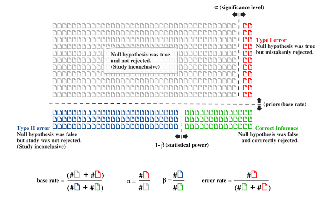
In this figure, the significance level was set at p < 0.05. But the error rate among conclusive studies is not 5%. It is 41.5%. Close to half of the conclusive studies in the diagram commit type I errors. This is despite the low significance level α=0.05 and the modest statistical power (1-β = 35%). Notice how decreasing statistical power (1-β) is like moving the dashed line between the green and blue area to the right. This will lead to a smaller green area and therefore a larger error rate. Likewise notice how increasing the base rate (i.e. testing more hypotheses that are unlikely to begin with) is like moving the horizontal dashed line down, resulting in more red, less green, and a higher rate of type I errors.
Note, the standard terminology can be very misleading. The “type I error rate” is defined as the rate of error among the cases where the null hypothesis is correct, rather than the rate of error among the cases where the null hypothesis was rejected. What we should be looking at is the error rate among the conclusive studies, i.e. studies that reject the null hypothesis.
Dodgy Rationalizations
It is often said that if you use p-values appropriately and do not misinterpret them, then all is fine. “Just understand what they mean and don’t draw inappropriate conclusions“. So what is a p-value supposed to mean then? How is it intended to be used?
What we call null-hypothesis testing is a hybrid between two [incompatible] approaches that are each fallacious by themselves: Fisher’s approach and the Neyman-Pearson approach.
Ronald Fisher, who popularized p-values, stated that p-values can be interpreted as “a rational and well-defined measure of reluctance to accept the hypotheses they test“. This statement is demonstrably false. Reluctance to accept a hypothesis should be measured by the probability of that hypothesis. And it is irrational to confuse inverse probabilities. Fisher interpreted p-values as a continuous measure of evidence against the null hypothesis, rather than something to be used in a test with a binary outcome.
The Neyman-Pearson approach, on the other hand, avoids assigning any interpretation to p-values. It, rather, proposes a “rule of behavior” for using p-values. One must reject the null hypothesis when its p-value fall below a predetermined threshold. They avoid the issue of inference and claim that this decision process leads to sufficiently low error rates in the long run.
But to rationalize p-values using a decision-making framework is absurd. Why would it matter what someone believes in if they behave indistinguishably from someone committing the conditional probability fallacy?
The rationale behind the Neyman-Pearson approach is that it is a method of hypothesis rejection that is “not too often wrong”. But this claim cannot be proven. If “wrong” is intended to mean “type I error”, then the error rate is no different than what we calculated above. If “wrong” means both types of errors then it is easy to show that the error rate can rise above alpha (the significance threshold).
Stop Trying to Salvage P-values
The concept of p-values is nearly a hundred years old. Despite the fact that its fundamental problem has been known, measuring significance remains the dominant method for testing statistical hypothesis. It is difficult to do statistics without using p-values and even more difficult to get published without statistical analysis of data.
However, things may be changing with the rise of the replication crisis in science [1, 2]. The extent to which the replication crisis can be attributed to the use of p-values is under debate. But the awareness about it has unleashed a wave of critisism and reconsideration of p-value testing.In 2016 the American Statistical Association published a statement saying: “Researchers often wish to turn a p-value into a statement about the truth of a null hypothesis or about the probability that random chance produced the observed data. The p-value is neither.” And in 2015 the Journal of Basic and Applied Social Psychology completely banned the use of p-values declaring that “The Null Hypothesis Significance Testing Procedure (NHSTP) is invalid” [3, 4].
Some have suggested abandoning statistical significance in favor of using continuous unthresholded p-values as a measure of evidence (Fisher’s approach) [5, 6, 7]. Others have suggested abandoning p-values as a continuous measure in favor of a dichotomous statistical significance (Neyman-Pearson’s approach) [8]. And others have suggested using more stringent thresholds for statistical significance [9]. But neither Fisher’s nor Neyman-Pearson’s approach are mathematically sound.
The mathematically sound approach is to abandon p-values, statistical significance, and null hypothesis testing all-together and to “to proceed immediately with other measures“, which is a “more radical and more difficult [proposal] but also more principled and more permanent“. (McShane et al 2018).
What alternatives do we have to p-values? Some suggest using confidence intervals to estimate effect sizes. Confidence intervals may have some advantages but they still suffer from the same fallacies (as nicely explained in Morey et al. 2016). Another alternative is to use Bayes factors as a measure for evidence. Bayesian model comparison has been around for nearly two decades but has not gained much traction, for a number of practical reasons.
The bottom line is that there is practically no correct way to use p-values. It does not matter if you understand what it means or if you frame it as a decision procedure rather than a method for inference . If you use p-values you are effectively behaving like someone that confuses conditional probabilities. Science needs a mathematically sound framework for doing statistics.
In future posts I will suggest a new simple framework for quantifying evidence. This framework is based on Bayes factors but makes a basic assumption: that every experiment has a probability of error that cannot be objectively determined. From this basic assumption a method of evidence quantification emerges that is highly reminescent of p-value testing but is 1) mathematically sound and 2) practical. (In contrast to Bayes factor, it produces numbers that are not extremely large or small).
Note: In an earlier version of this post I had “The type I error rate is defined as the rate of error among the cases where the null hypothesis is incorrect, rather than the rate of error among the cases where the null hypothesis was rejected” which is now corrected to “rate of error among the cases where the null hypothesis is correct“. I want to thank Richard O’Farrell for catching this mistake.
My intuitive explanation of what I see as the heart of your argument is as follows. If your experiment result R is unlikely in the world where H0 is true, but *also* unlikely in the world where H0 is false, then observing R is not good evidence against H0. In fact, if R is *even more* unlikely in the world where H0 is false than the one where it’s true, it could be evidence *for* H0.
Is that a correct summary/gloss of the problem?
Yes! Precisely. Although that’s one of the two sources of invalid hypothesis rejection. Another source is the priors. If H0 is already very likely, prior to seeing R, then you need more evidence to justify rejecting H0. See this wiki link for an illustrative example (the breathalyzer tests) https://en.wikipedia.org/wiki/Base_rate_fallacy#Example_2:_Drunk_drivers
We do rely too much on this kind of analysis, especially in industry because money usually follows log-normal, meaning a few elements who have the highest impact dominate the outcome, regardless of the size of the population.
Exited to read more.